
CS194-26 Final Projects
Ja (Thanakul) Wattanawong and Briana Zhang
Poor Man’s Augmented Reality
In this project, we project a cube onto the center of the face of a rubrik’s cube by calculating the calibration matrix of the camera through known 3D coordinates of each image we are projecting on.
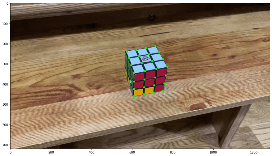
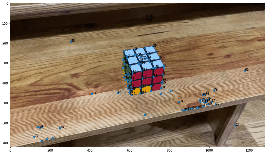
The first step we needed to take for our baby AR is to find a set of known 3D world coordinates. For precision, we calculated harris corner points of our rubrik’s cube and selected the points we wanted.
Due to the perfect shape of the cube, we were easily able to correspond each 2D point to a 3D point by going through the green points in row-major order. We defined the bottom left most point as the origin, up as the z-axis, right as x-axis, and vertical but in the flat plane as the y-axis.
The next step was to continuously detect these points for every image. Rather than selecting the harris corner points again every time, we used the in-built MedianFlow tracker of the cv2 package. This tracked the above green points throughout the video.
As you can see, this was mostly good, though it did drift for some points.
With the correspondances to 3D coordinates, we were able to calculate the calibration matrix of each image. The calibration matrix essentially calculates what transformation is necessary from 3D to 2D in a particular image. This requires having at least 8 points, with the 9th parameter of the matrix set to 1.
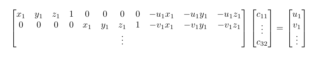
The particular method we used to calculate the calibration matrix was using least squares on the below matrix.
We did not use RANSAC because our results without it were fairly good. Below is an example of the calibration matrix applied to our original 3D points. It looks better than the original points chosen via harris corners.
After calculating the calibration matrix of every image, we were able to project a cube by calculating the 3D coordinates of the cube and applying the calibration matrix to those points.
Finally, we used a draw function that was in an open cv tutorial for drawing the cube in a more interesting manner. We applied this for two videos.
Lightfield Camera
In this project we used various images taken in a light field array to create cool effects.
Here I used the method described here in order to scale and shift the images such that the image can focus at different depths by varying the parameter  in the range of
  . Here are animated gifs of chess and amethyst scenes moving in focus:
In this part we simulated aperture adjustment by averaging images from cameras that were within radius  of a point (we used the mean of u,v) in order to simulate aperture changes to vary how much background was blurred out. Here are gifs of the aperture increasing which simulates depth of field:
I learned a lot about how great effects can be emulated when you have a large number of images in a light field arrangement. It’s a shame the technology did not take off and become commonplace.
Image Quilting
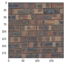
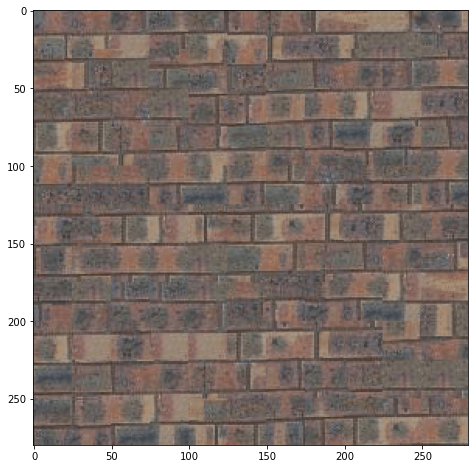
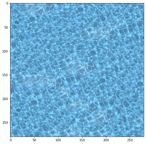
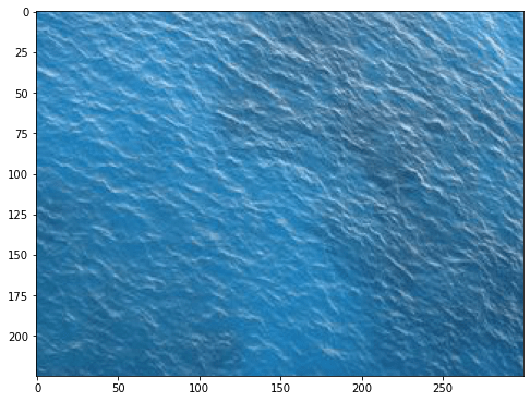
This project illustrates a couple of methods that were used for texture synthesis and transfer and shows some of their effects. The three methods under comparison are random sampling, overlap, and seam finding with explanation as follows:
This part involves sampling random square patches from the original texture, which resulted in a lot of edge artifacts
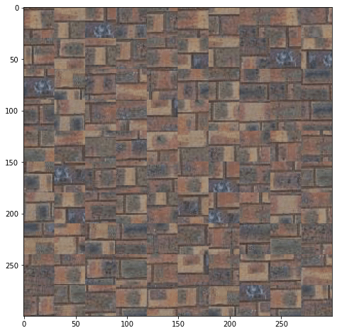
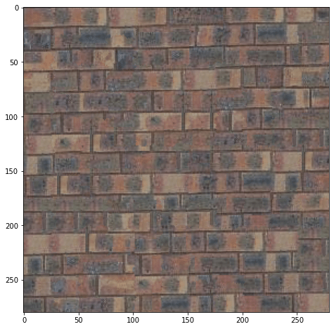
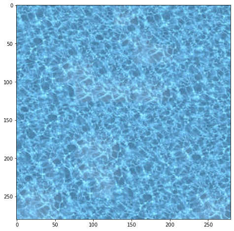
This next part samples overlapping patches that were chosen to minimize the SSD error in the overlapping regions. I chose to randomly sample from the 5 lowest cost patches to provide interesting stochasticity while still having good overlap cost.
After this we wrote a dynamic programming routine in Python using the paper’s algorithm to find the minimum cost path through the overlapping region, which was very helpful in eliminating edge artifacts. (Bells & Whistles)
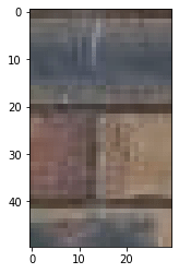
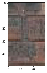
Brick Texture | Random Sampling |
Overlap | Seam Finding |
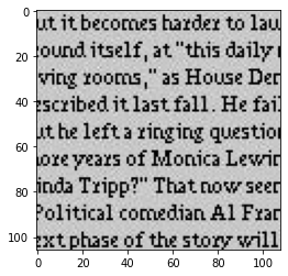
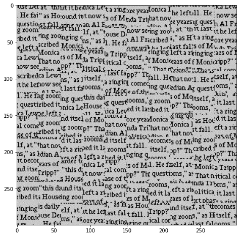
Text Texture | Random Sampling |
Overlap | Seam Finding |
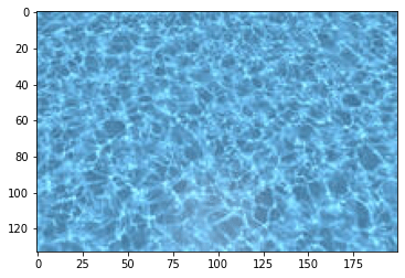
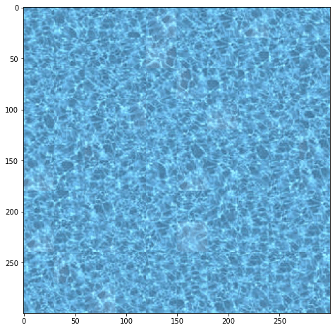
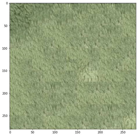
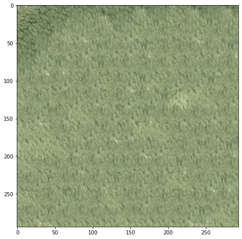
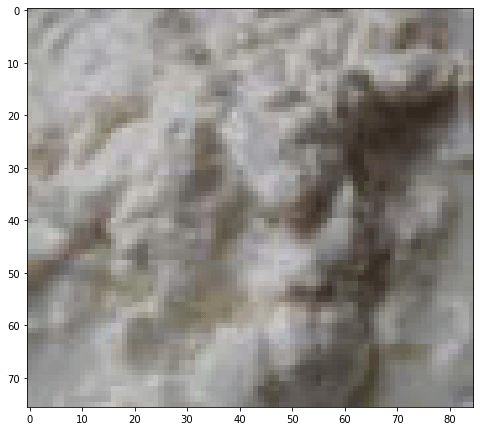
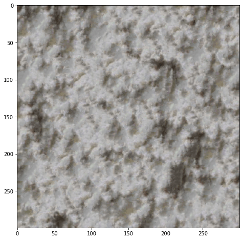
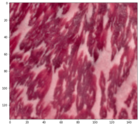
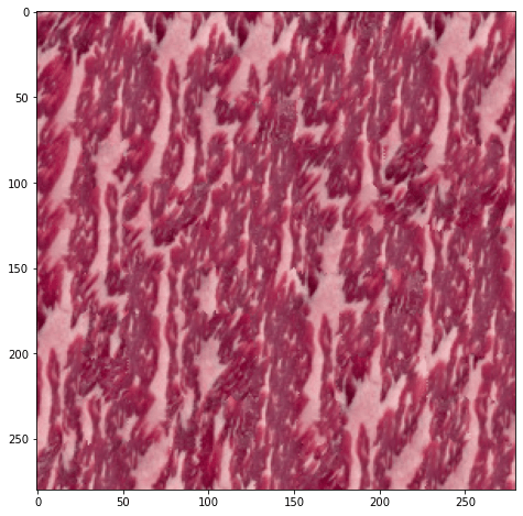
Texture | Random Sampling |
Overlap | Seam Finding |
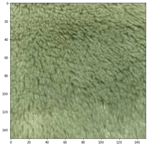
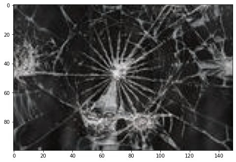
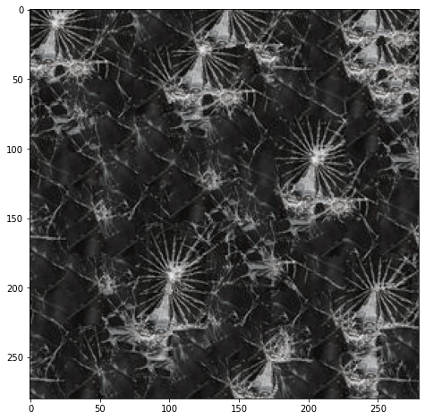
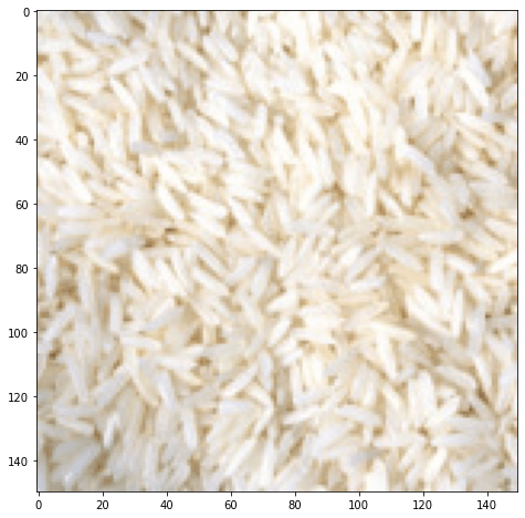
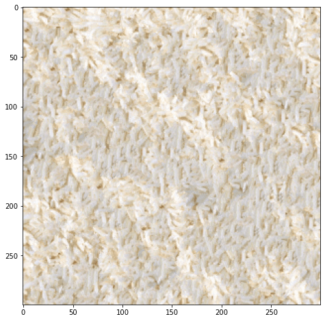
Texture | Random Sampling |
Overlap | Seam Finding |
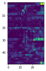
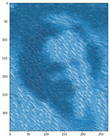
For seam finding, what we did was start with two overlapping patches and the error patch between them (SSD):
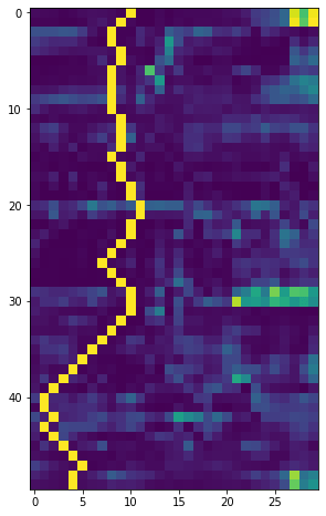
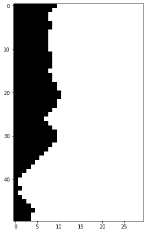
Then, we computed the min-cost path through the cost image using dynamic programming, which looks like the following:
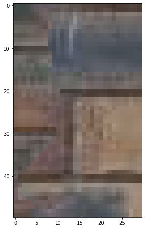
Min-cost path | Mask | Final Result |
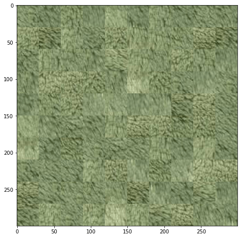
By using this min-cost seam-finding subroutine, we are able to construct the image quilting texture synthesis method. First, we used the code for choose_sample to ensure that the overlap cost for the candidate image was low, and the code is very similar to quilt_simple except that where we would replace the output image with the new patch, we used the seam-finding subroutine to mask the best path through and reduce edge artifacts that could result from harsh color changes. Here are four more examples demonstrating this seam-finding texture synthesis method:
Original | Synthesized |
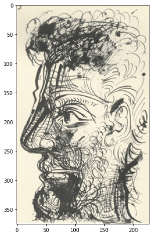
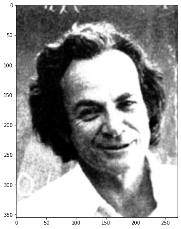
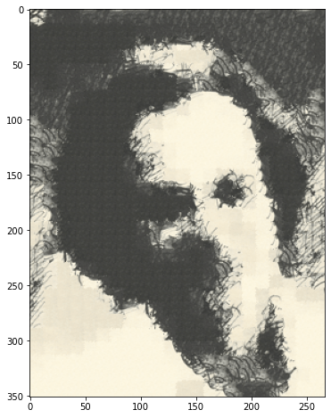
For texture transfer we used the grayscale version of the images to represent luminance, creating a correspondence map and an additional cost term. This allows texture to be transferred onto another image. We tried various alphas, deciding on a lower alpha of 0.4 in order to favor texture over blending.
Sample | Target | Transferred |